This is the 5th part of my LibreOffice Tutorial to learn about simple useful formulas and a tiny bit of macro to make a simple daily agenda.
Other parts:
In Part 1 we look at renaming a sheet, entering some random data, formatting cells and starting to build the logic of the agenda.
In Part 2 of this tutorial we write some time functions and IF formulas.
In Part 3 of this tutorial we learn about nested IF and AND function.
In Part 4 of this tutorial we learn about VLOOKUP.
In Part 5 we look at how to create and use a ‘named range’.
In Part 6, we learn the INDEX function.
In Part 7, we learn how to code a (very) simple LibreOffice Macro.
In Part 8, we use the MROUND function to round the time.
In Part 9 part we do some debugging and learned about the ISERROR and NOT functions.
In Part 10 part we add some color and formatting to wrap-up this series.
In this fifth episode of the Tutorial series, we are going to learn how to create and use a named range.
In cell C8 of sheet ‘Now!’ we have the following formula:
=VLOOKUP(1,$planner.A2:D9,4,)
It does display the current activity, so our reference to $planner.A2:D9 works fine. If not and you need some help, please leave a comment to this article and I’ll help you to solve the issue.
Let’s display in cell D8 the start time corresponding to the current activity, and in E8 the end time.
We can simply drag cell C8 two cells to the right. We are getting this:

The activity is fine (“Finally free!”) but I am getting an #N/A error in D8 and nothing in E8.
The #N/A error is happening because the VLOOKUP function is searching for the value 1 and cannot find it at all.
If you look at the formula that is in D8 and E8 now, you will realise that the reference to the cell range has changed and because of that we need to amend the formula in both cells:
| Row \ Colum | C | D | E |
| 8 | ‘=VLOOKUP(1,$planner.A2:D9,4,) | ‘=VLOOKUP(1,$planner.B2:E9,4,) | ‘=VLOOKUP(1,$planner.C2:F9,4,) |
There are two things we want to change in D8 and E8:
In both cells the reference to the table containing the activity, start time and end time, located in sheet ‘planner’ is not right. Indeed by dragging the cell to the right, the reference has also changed from A2:D9 to B2:E9, and to C2:F9.
We could have locked the reference with ‘$’ (dollar sign) in cell C8 before dragging the formula to the right, as seen in part 2.
So our cell in C8 would be:
=VLOOKUP(1,$planner.$A2:$D9,4,)
This would solve our problem, but imagine that would want to add a new activity, like “walk to the park”, in the list of activities you then would need to change the table reference in every cell using the table.
That is why named range are used for: once you have defined a named range with reference to a table like $planner.$A2:$D9, you can use the named range in the cells that need to use that table, like our D8 and E8. And whenever you want to extend the table with a new line or a new column you can easily update the named range, and you don’t need to update all the cells using that named range.
And it is very easy to create a named range!
And this is how to do it.
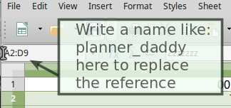
In our sheet named ‘planner’, select the cells region from A2 to D9. Then in the top left corner, just above the column numbers, where you can see the reference of the selection, write something like ‘planner_daddy’ there, and press enter. That’s it, your range A2:D9 has been named!
There are a few restriction on the name that you can give, for example you cannot name it ‘planner’ because there is a sheet already with this name and that would be confusing for LibreOffice…
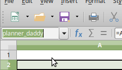
So to make sure it works, click anywhere in the sheet to deselect your table. Then select the name you have entered from the drop down list in that same corner, and if everything is fine it should highlight your table
Son back to our sheet named ‘Now!’,we can now replace the formula in C8 with:
=VLOOKUP(1,planner_daddy,4,)
Then you can drag C8 to D8 and E8.
We are not finished yet. To get the ‘start time’ in D8, we simply need to replace the ‘4’ in the formula with ‘2’, because this is the column number of the ‘start time’ column in table ‘planner_daddy’.
Similarly in E8 you simply need to replace the ‘4’ with ‘3’, which is the column number for ‘end time’ in ‘planner_daddy’ table.
So we should have the following formulas:
| Row/Column | C | D | E |
| 8 | ‘=VLOOKUP(1,planner_daddy,4,) | ‘=VLOOKUP(1,planner_daddy,2,) | ‘=VLOOKUP(1,planner_daddy,3,) |
And I have the following display:

And I feel so tired now!
In the next part of this LibreOffice Tutorial I will show you how to display the previous and next activities using function INDEX().
(to be continued)
If you like this tutorial you could buy me a coffee to help me continue writing add-free tutorials.
Thank you!
Related Posts
 LibreOffice Calc & Python: part 9 – Reverse the order of cells content from a cell range
 LibreOffice Calc & Python Programming: part 8 – From Python Tuple to Cells Range
 LibreOffice Calc & Python Programming: part 7 – From Cells Range to Python Tuple.
- LibreOffice Calc & Python Programming: part 6 – Type of a Cell content.
 LibreOffice Calc & Python Programming: Annex 1 – Assign a Python Macro to a key.
 LibreOffice Calc & Python Programming: Part 5 – display a message window.
Please help!
How do i do a dynamic name range in libre office calc spreedsheet.
I have been unable to the offset function to work.
I have been working on this for a mothh. A solution will be greatly appreciated.
The number of rows in column A increases with new entries. I need the name range to increase also.
Hi Will, and thanks for your question. As an example I have in Column A: A1:”Fruits”, A2:”Apple”,A3:”Cherry”,A4:”Pear”. In the ‘Managed Names’ Window, click on the ‘Add’ button, then enter as name ‘fruits’, then in the ‘Range or formula expression’ enter “OFFSET($A$2,0,0,COUNTA($A:$A)-1,1)”(without the quotes).
The COUNTA($A:$A)-1 counts all the cells with a value in the column A, minus 1 to exclude the header in A1 (“Fruits”), if you don’t put any header you can omit the ‘-1’. The OFFSET here is simply returning a range with a height of n rows, n being the number of values in column A -1, and a width of 1 Column, with the top-left cell being at $A$2 with no offset (0,0).
Now in any other column you can access the elements of the named range with “=INDEX(fruits,2)” -> Cherry. The range will expand when adding e.g. “Banana” in Cell A5.To verify the number of values listed in the range ‘fruits’, you can do “=COUNTA(fruits)” in any cell and see it growing when you add a new fruit in the list. And as a proof that it is not simply counting the non-empty cells in column A, try in a cell “=INDEX(fruits;5) and you’ll get a ‘#Ref’ error because there is no elements at index 5 of the ‘fruits’ range.
It is confusing because the named range will not appear in the ‘Name Box’ drop down list, but you can still access it. Aso, when selecting the name ‘fruits’ in the ‘Manage Names’ window it will refer to the entire Column A). Another example is to select a cell (outside your range’s column) and go in “Data/Validity”, then select ‘Cell Range’ and enter ‘fruits’ in the name of the cell range. The cell will then be populated with a drop down list bound to your ‘fruit’ named range.
I am calling it a named range, but it is actually only a cell range with a reference hence it not being displayed in the ‘Name Box’ or in the ‘Range names’ section in the Navigator.
Please let me know if that answers you question. Cheers